Convert British to US Dates

The below video shows you how to convert from British to US dates automatically with VBA code in Excel 2007, 2010, and 2013. The code also works the other way and will convert from US dates to British date format. This Excel tutorial will teach you how to use the =mid, =left, =search, and =right formulas to modify dates quickly in Excel.

Please select the gear icon at the bottom right of the Youtube video and switch the quality to 1080P HD for the best viewing experience.

If you are on mobile, I recommend watching the video directly on My Youtube for best video quality.

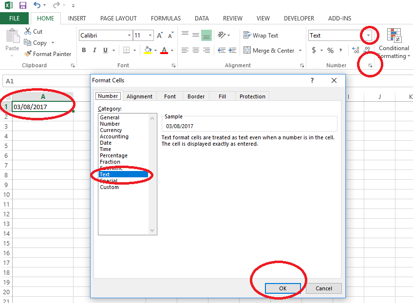
For the below examples, please work with 03/08/2017. Please Note: convert the cell to a text data type before using these formulas to work on the cell. You can do that by selecting the cell and selecting text from the drop-down box:

Explanation of =MID Formula
=MID(text, start_num, num_chars)
text: The reference cell. For example, cell A1.
start_num: The character that you want to begin from. For the following string 2017, 2 is the first character, 0 is the 2nd character, 1 is the 3rd character, and 7 is the 4th character. If you want to return only 17, then do =mid(A1,3,2).
num_chars: How many of the characters you want to return. In the above example =mid(A1,3,2), you want to return 2 characters 1 & 7.

Explanation of =RIGHT Formula
=RIGHT(text, number of characters)
text: The reference cell. For example, cell A1.
num_chars: How many of the characters you want to return. In the string 03082017, if you wanted to return only 2017, then the formula would be =Right(A1, 4)

Explanation of =LEFT Formula
=LEFT(text, number of characters)
text: The reference cell. For example, cell A1.
num_chars: How many of the characters you want to return. In the string 03082017, if you wanted to return only 03, then the formula would be =Left(cell source, 2)

Explanation of =SEARCH Formula
=SEARCH(find_text, within_text, [start_num])
find_text: If you want to find the character number of the first / in the string 03/18/2017, then you would put "/" in the find_text argument.
within_text: The reference cell. For example, cell A1.
[start_num]:The character that you want to begin from. For the following string 03/18/2017, =search("/",A1,1) would return the value 3 being that / is the third character in the string 03/18/2017. If, on the other hand, you want to return the character position of the second /, then you would use the formula =search("/",A1,4). By putting 4 as the starting number, you are starting from 1 and searching for the first / that appears after 1. If 1 were to instead be a /, then it would return 4. The formula =search("/",A1,4) returns 6 for the string 03/18/2017 since the position of the 1st / beginning on and including character 4 is character position 6.

VBA Convert British to US Date Format

Sub BritishtoUSDates()

erow = ActiveSheet.Cells(Rows.Count, 1).End(xlUp).Row

Columns("B:B").Select
ActiveCell.FormulaR1C1 = "=isnumber(RC[-1])"
Range("B1").Select
Selection.AutoFill Destination:=Range("B1:B" & erow), Type:=xlFillDefault

Columns("B").Select
Selection.Copy
Columns("B").Select
Selection.PasteSpecial Paste:=xlPasteValues, operation:=xlNone, skipblanks _
:=False, Transpose:=False

Columns("B:B").Select
Selection.TextToColumns Destination:=Range("B1"), DataType:=xlDelimited, _
textqualifier:=xlDoubleQuote, consecutivedelimiter:=False, Tab:=True, _
semicolon:=False, comma:=False, Space:=False, other:=False, fieldinfo _
:=Array(1, 2), trailingminusnumbers:=True

Range("C1").Select
ActiveCell.FormulaR1C1 = "=if(RC[-1]=""FALSE"",1,0)"
Range("c1").Select
Selection.AutoFill Destination:=Range("C1:C" & erow), Type:=xlFillDefault

Columns("C").Select
Selection.Copy
Columns("C").Select
Selection.PasteSpecial Paste:=xlPasteValues, operation:=xlNone, skipblanks _
:=False, Transpose:=False

Dim y As Integer
y = 1
erow = erow + 1

Do Until y = erow

If Range("C" & y).Value = 0 Then
Range("A" & y).Value = Range("A" & y).Value & "B"
End If
y = y + 1

Loop

Columns("A").Select
Selection.Copy
erow = erow − 1

Range("d1").Select
ActiveCell.FormulaR1C1 = "=search(""/"",RC[-3],1)"
Range("D1").Select
Selection.AutoFill Destination:=Range("D1:D" & erow), Type:=xlFillDefault
Range("E1").Select
ActiveCell.FormulaR1C1 = "=search(""/"",RC[-4],4)"
Range("E1").Select
Selection.AutoFill Destination:=Range("E1:E" & erow), Type:=xlFillDefault
Columns("D:E").Select
Selection.Copy
Columns("D:E").Select
Selection.PasteSpecial Paste:=xlPasteValues, operation:=xlNone, skipblanks _
:=False, Transpose:=False
Columns("A").Select
Selection.Copy
Columns("F").Select
Selection.PasteSpecial Paste:=xlPasteValues, operation:=xlNone, skipblanks _
:=False, Transpose:=False

y = 1
Dim drum As Integer
Dim drum2 As Integer

erow = erow + 1

Do Until y = erow
drum = Range("D" & y).Value
drum2 = Range("E" & y).Value

Select Case drum
Case Is = 3
Select Case drum2
Case Is = 6
Range("I" & y).Select
ActiveCell.FormulaR1C1 = "=concatenate(MID(RC[-3],4,2),""/"",LEFT(RC[-3],2),""/"",mid(RC[-3],7,4))"
Case Is = 5
Range("i" & y).Select
ActiveCell.FormulaR1C1 = "=concatenate(MID(RC[-3],4,1),""/"",LEFT(RC[-3],2),""/"",MID(RC[-3],6,4))"
End Select
Case Is = 2
Select Case drum2
Case Is = 4
Range("i" & y).Select
ActiveCell.FormulaR1C1 = "=concatenate(MID(RC[-3],3,1),""/"",LEFT(RC[-3],1),""/"",MID(RC[-3],5,4))"
Case Is = 5
Range("i" & y).Select
ActiveCell.FormulaR1C1 = "=concatenate(MID(RC[-3],3,2),""/"",LEFT(RC[-3],1),""/"",MID(RC[-3],6,4))"
End Select
End Select
y = y + 1
Loop

Columns("i").Select
Selection.Copy
Columns("i").Select
Selection.PasteSpecial Paste:=xlPasteValues, operation:=xlNone, skipblanks _
:=False, Transpose:=False

Columns("a:h").Select
Selection.Delete

End Sub