Free VBA Book
The below images contain a free VBA book I wrote about coding with Excel. It's a modern programming language that has worked with Microsoft Office since before Windows 7 and Microsoft Office 2007. The language doesn't change as computers are upgraded.
VBA is the most secure programming language that requires no installation. VBA can execute millions of computer actions and calculations in seconds.
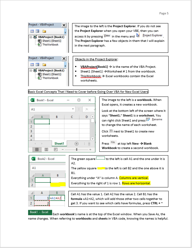

Visual Basic Editor (VBE)
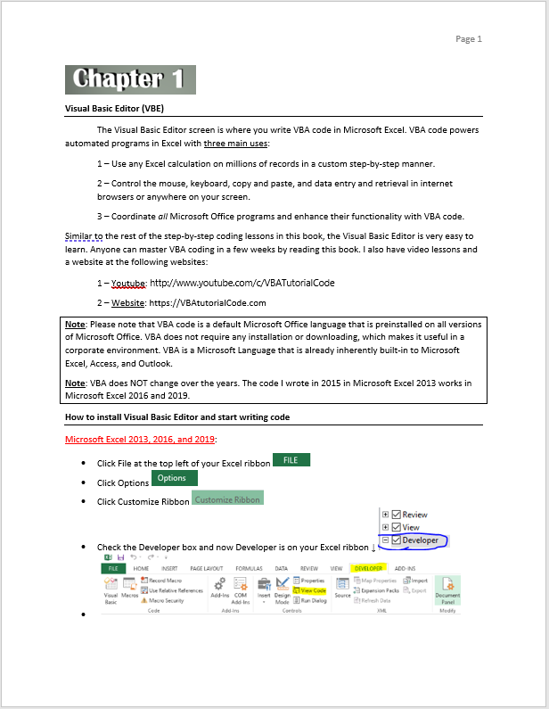
The Visual Basic Editor screen is where you write VBA code in Microsoft Excel. VBA code powers automated programs in Excel with three main uses:
1 – Use any Excel calculation on millions of records in a custom step-by-step manner.
2 – Control the mouse, keyboard, copy and paste, and data entry and retrieval in internet browsers or anywhere on your screen.
3 – Coordinate all Microsoft Office programs and enhance their functionality with VBA code.
Similar to the rest of the step-by-step coding lessons in this book, the Visual Basic Editor is very easy to learn. Anyone can master VBA coding in a few weeks by reading this book. I also have video lessons and a website at the following websites:
1 – Youtube: http://www.youtube.com/c/VBATutorialCode
2 – Website: https://VBAtutorialCode.com
Note: Please note that VBA code is a default Microsoft Office language that is preinstalled on all versions of Microsoft Office. VBA does not require any installation or downloading, which makes it useful in a corporate environment. VBA is a Microsoft Language that is already inherently built-in to Microsoft Excel, Access, and Outlook.
Note: VBA does NOT change over the years. The code I wrote in 2015 in Microsoft Excel 2013 works in Microsoft Excel 2016 and 2019.
How to install Visual Basic Editor and start writing code
Microsoft Excel 2013, 2016, and 2019:
- Click File at the top left of your Excel ribbon
- Click Options
- Click Customize Ribbon
- Check the Developer box and now Developer is on your Excel ribbon ↓
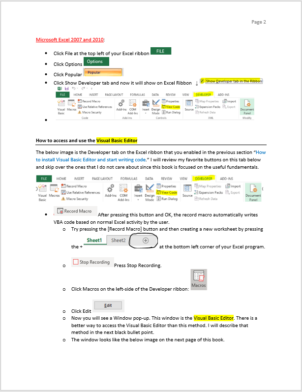
Microsoft Excel 2007 and 2010:
- Click File at the top left of your Excel ribbon
- Click Options
- Click Popular
- Click Show Developer tab and now it will show on Excel Ribbon ↓
How to access and use the Visual Basic Editor
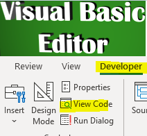
The below image is the Developer tab on the Excel ribbon that you enabled in the previous section “How to install Visual Basic Editor and start writing code.” I will review my favorite buttons on this tab below and skip over the ones that I do not care about since this book is focused on the useful fundamentals.
After pressing this button and OK, the record macro automatically writes VBA code based on normal Excel activity by the user.
- Try pressing the [Record Macro] button and then creating a new worksheet by pressing the +
at the bottom left corner of your Excel program.
Press Stop Recording.
- Click Macros on the left-side of the Developer ribbon:
- Click Edit
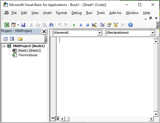
- Now you will see a Window pop-up. This window is the Visual Basic Editor. There is a better way to access the Visual Basic Editor than this method. I will describe that method in the next black bullet point.
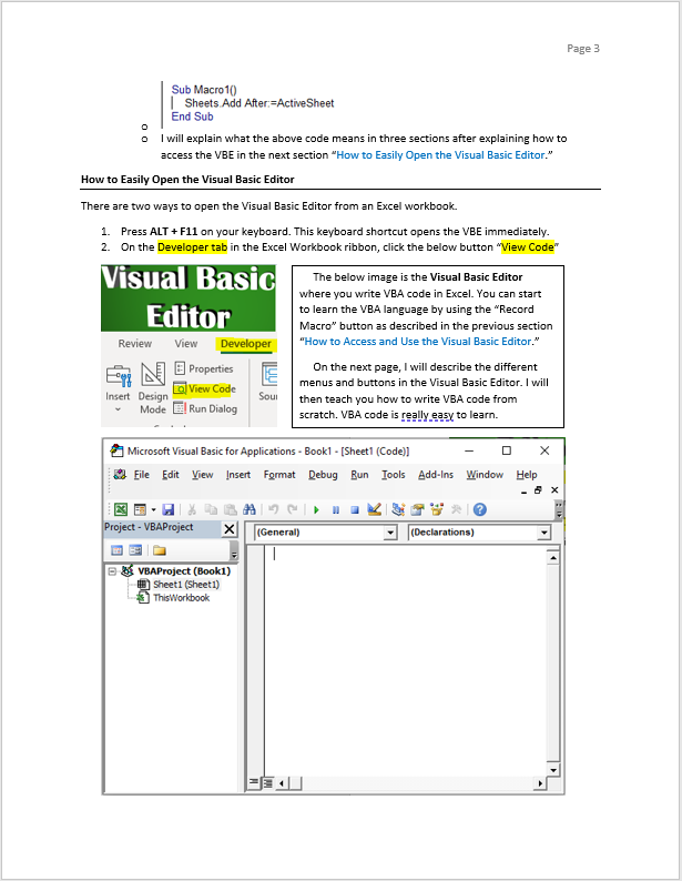
- The window looks like the below image on the next page of this book.
- I will explain what the above code means in three sections after explaining how to access the VBE in the next section “How to Easily Open the Visual Basic Editor.”
How to Easily Open the Visual Basic Editor
There are two ways to open the Visual Basic Editor from an Excel workbook.
- Press ALT + F11 on your keyboard. This keyboard shortcut opens the VBE immediately.
- On the Developer tab in the Excel Workbook ribbon, click the below button “View Code”

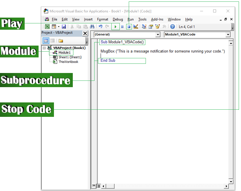
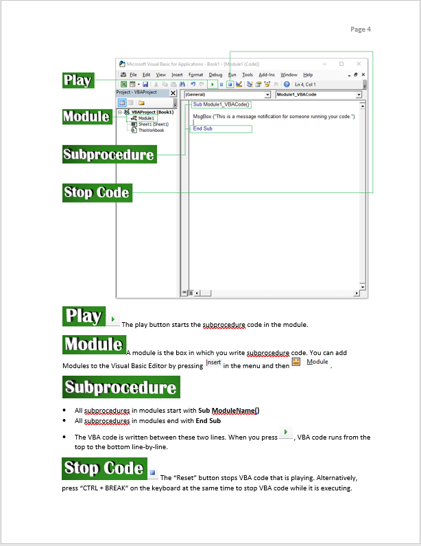
The play button starts the subprocedure code in the module.
A module is the box in which you write subprocedure code. You can add Modules to the Visual Basic Editor by pressing
in the menu and then
.

- All subprocedures in modules start with Sub ModuleName()
- All subprocedures in modules end with End Sub
- The VBA code is written between these two lines. When you press
, VBA code runs from the top to the bottom line-by-line.
The “Reset” button stops VBA code that is playing. Alternatively, press “CTRL + BREAK” on the keyboard at the same time to stop VBA code while it is executing.


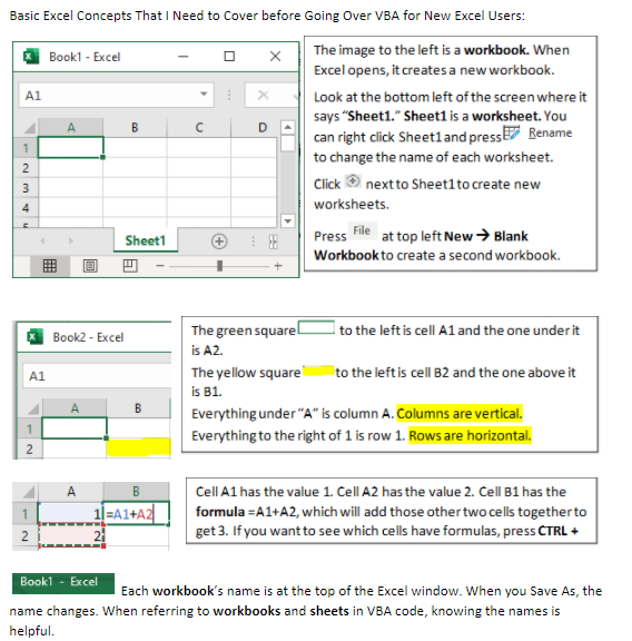

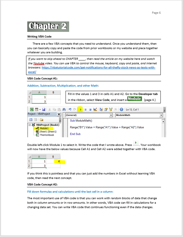
Writing VBA Code
There are a few VBA concepts that you need to understand. Once you understand them, then you can basically copy and paste the code from prior workbooks or my website and piece together whatever you are building.
VBA Code Concept #1:
Addition, Subtraction, Multiplication, and other Math:


Double left-click Module 1 to select it. Write the code that I wrote above. Press . Your workbook will now have the below values because Cell A1 and Cell A2 were added together with VBA code.

If you think this is pointless and that you can just add the numbers in Excel without learning VBA code, then read the next concept.
VBA Code Concept #2:
Fill down formulas and calculations until the last cell in a column:
The most important use of VBA code is that you can work with random blocks of data that change both in column amounts or in row amounts. In other words, VBA code can fill in calculations for a changing data set. You can write VBA code that continues functioning even if the data changes.
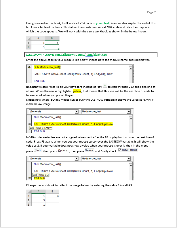
Going forward in this book, I will write all VBA code in green text. You can also skip to the end of this book for a table of contents. This table of contents contains all VBA code and cites the chapter in which the code appears. We will work with the same workbook as shown in the below image:

LASTROW = ActiveSheet.Cells(Rows.Count,1).End(xlUp).Row
Enter the above code in your module like below. Please note the module name does not matter.

Important Note: Press F8 on your keyboard instead of Play to step through VBA code one line at a time. When the row is highlighted yellow, that means that this line will be the next line of code to be executed when you press F8 again.
Notice how when I put my mouse cursor over the LASTROW variable it shows the value as “EMPTY” in the below image.

In VBA code, variables are not assigned values until after the F8 or play button is on the next line of code. Press F8 again. When you put your mouse cursor over the LASTROW variable, it will show the value as 2. If your variable does not show a value when your mouse is over it, then in the menu press , then press
, then press
, and finally check
.

Change the workbook to reflect the image below by entering the value 1 in cell A3:

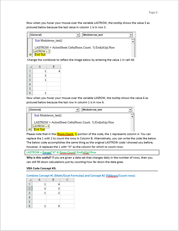
Now when you hover your mouse over the variable LASTROW, the tooltip shows the value 3 as pictured below because the last value in column 1 is in row 3.

Change the workbook to reflect the image below by entering the value 1 in cell A6:
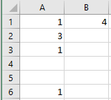
Now when you hover your mouse over the variable LASROW, the tooltip shows the value 6 as pictured below because the last row in column 1 is in row 6.

Please note that in the (Rows.Count, 1) portion of the code, the 1 represents column A. You can replace the 1 with 2 to count the rows in Column B. Alternatively, you can write the code like below. The below code accomplishes the same thing as the original LASTROW code I showed you before; however, it replaces the 1 with “A” as the column for which to count rows:
LASTROW = Range("A" & Rows.Count).End(xlUp).Row
Why is this useful? If you are given a data set that changes daily in the number of rows, then you can still fill down calculations just by counting how far down the data goes.
VBA Code Concept #3:
Combine Concept #1 (Math/Excel Formulas) and Concept #2 (Filldown/Count rows):
Go to ,
,
, and check
.
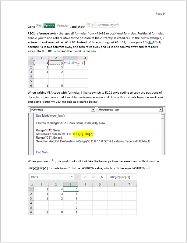
R1C1 reference style – changes all formulas from =A1+B1 to positional formulas. Positional formulas enable you to add cells relative to the position of the currently selected cell. In the below example, I entered = and selected cell A1 + B1. Instead of Excel writing out A1 + B1, it now puts RC[-2]+RC[-1] because A1 is two columns away and zero rows away and B1 is one column away and zero rows away. The R in RC is row and the C in RC is column.
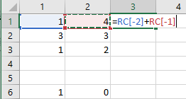
When writing VBA code with formulas, I like to switch to R1C1 style coding to copy the positions of the columns and rows that I want to use formulas on in VBA. I copy this formula from the workbook and paste it into my VBA module as pictured below:
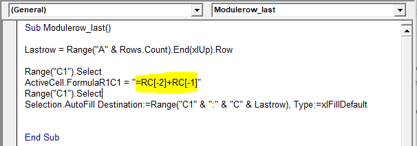
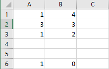
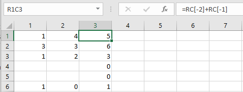
When you press , the workbook will look like the below picture because it auto-fills down the
=RC[-2]+RC[-1] formula from C1 to the LASTROW value, which is C6 because LASTROW = 6.
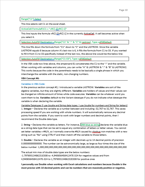
Range("C1").Select
This line selects cell C1 on the excel sheet.
ActiveCell.FormulaR1C1 = "=RC[-2]+RC[-1]"
This line inputs the formula =RC[-2]+RC[-1] in the currently ActiveCell. A cell becomes active when you select it.
Selection.AutoFill Destination:=Range("C1" & ":" & "C" & Lastrow), Type:=xlFillDefault
This line fills down the formula from “C1” down to “C” and the LASTROW. Since the variable LASTROW equals 6 because column A’s last row is 6, it fills the formula from C1 to C6. If you wanted to fill it from C1 to C6 specifically instead of the last row, the above line would be the below line:
Selection.AutoFill Destination:=Range("C1:C6"), Type:=xlFillDefault
In the VBA code two lines above, the ampersand & concatenates the C1 to the “:” and the variable. When working with variables and columns, you can write “A” & LASTROW & “:” & “B” & LASTROW2. This works because the code in the parenthesis needs to be basically a single phrase in which you interchange the variable with the static, non-changing numbers.
VBA Concept #4:
Variables in VBA Code and String Variable Datatype:
In the previous section concept #3, I introduced a variable LASTROW. Variables are sort of like algebra variables, but they are slightly different. Variables are holders of values and their values can be changed an infinite amount of times while code executes. Variables can be whatever word you want them to be. Variables default to the Variant datatype if you do not indicate what datatype the variable is when declaring the variable.
Variable Datatypes (I use Double and String data types. I use Double for numbers and String for letters)
1. Integer – Declares the variable as a number between and including -32,767 to 32,767. This saves processing speed if you are working with whole numbers. It will automatically remove any decimal points from the variable. If you want to work with larger numbers and decimal points, then I recommend the Double data type.
2. String – Declares the variable as letters. For instance, DIM blue as string declares the variable blue as a string data type that can be set to equal any combination of letters or letter values. You cannot set letter variables = #N/A, so I normally overwrite #N/A caused by vlookup non-matches with a new string such as "No" using CTRL+F and then match off the variable to those letters.
3. Double – Declares the variable as an integer with decimals up to 14 decimal points of precision 0.00000000000000. The number can be astronomically large, as large as four times the size of the below number: 1,000,000,000,000,000,000,000,000,000,000,000,000,000,000,000,000,000,000,000
The actual min max of double data types are the below numbers:
-1.79769313486231E308 to -4,94065645841247E-324 for negative values and from 4,94065645841247E-324 to 1,79769313486232E308 for positive ones
I personally use Double when working with Excel calculations and numbers because Double is the most precise with 14 decimal points and can be numbers that are massively positive or negative.
4. Long – Long is the same as the Integer datatype. The only difference is that Long rounds up or down to nearest whole number. For Long variables, if the variable is equal to 3.5 then it will process as 4. If the variable is 3.4, then it will process as 3. The integer straight up removes the decimal point without concern for rounding. The integer datatype always rounds down.
5. Date – Lets you declare a date variable such as June 19, 2017.
6. There are other datatypes, but for the purpose of this book I will not cover them.
VBA Concept #5:
Declaring Variables and Assigning Values to Variables Part 1:
DIM statement – the most frequently used way to declare a variable in VBA code at the module level.
String Datatype example:
Dim variable1 as string à declares variable1 as a string variable.
Variable1 = “Subscribe"
The above sets variable1 equal to the text value “Subscribe"
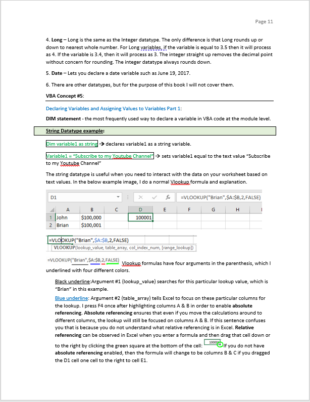
The string datatype is useful when you need to interact with the data on your worksheet based on text values. In the below example image, I do a normal Vlookup formula and explanation.


Vlookup formulas have four arguments in the parenthesis, which I underlined with four different colors.
Black underline:Argument #1 (lookup_value) searches for this particular lookup value, which is “Brian” in this example.
Blue underline: Argument #2 (table_array) tells Excel to focus on these particular columns for the lookup. I press F4 once after highlighting columns A & B in order to enable absolute referencing. Absolute referencing ensures that even if you move the calculations around to different columns, the lookup will still be focused on columns A & B. If this sentence confuses you that is because you do not understand what relative referencing is in Excel. Relative referencing can be observed in Excel when you enter a formula and then drag that cell down or to the right by clicking the green square at the bottom of the cell: If you do not have absolute referencing enabled, then the formula will change to be columns B & C if you dragged the D1 cell one cell to the right to cell E1.
Red underline: Argument #3 (col_index_num) tells Excel which column you want to return once Excel finds the value from Argument #1. In my example, I used 2 so that I could get the value from column 2 or B next to the value Brian. Vlookups are limited in that you can only get one value from a vlookup but there are workarounds such as sorting and concatenating columns with VBA to match based off of more criteria or using SUMPRODUCT similar to how I do in the last 3 minutes of this video: https://www.youtube.com/watch?v=PkHbJ3fsfK8
Green underline: Argument #4 (optional) – I use FALSE to indicate that it is an exact match. I never use TRUE because it’s so uncertain and unintentional.
I know I went on a tangent here explaining VLOOKUP formulas but everyone should know about them. Now I will explain how VBA can be used with string data types to work around data issues.

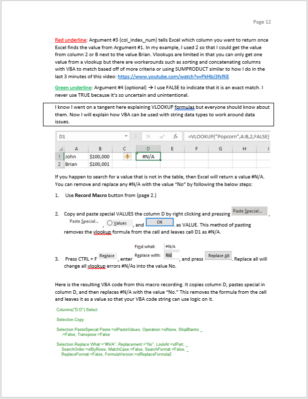
If you happen to search for a value that is not in the table, then Excel will return a value #N/A. You can remove and replace any #N/A with the value “No” by following the below steps:
- Use Record Macro button from (page 2.)
- Copy and paste special VALUES the column D by right clicking and pressing
,
,
, and
. as VALUE. This method of pasting removes the vlookup formula from the cell and leaves cell D1 as #N/A.
- Press CTRL + F
, enter
, and press
. Replace all will change all vlookup errors #N/As into the value No.
Here is the resulting VBA code from this macro recording. It copies column D, pastes special in column D, and then replaces #N/A with the value “No.” This removes the formula from the cell and leaves it as a value so that your VBA code string can use logic on it.

I know I went on another tangent here about replacing #N/A values with VBA code, but this concept is important when looping through VBA code. Now I will tie this whole monologue back to string variables by also introducing VBA loops. After I explain VBA loops, I’ll introduce double variables.
VBA Concept #6:
VBA Loops and Double Variable Datatype:
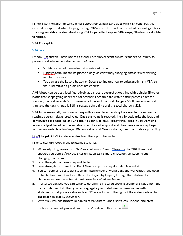
By now, I’m sure you have noticed a trend. Each VBA concept can be expanded to infinity to process basically an unlimited amount of data:
- Variables can hold an unlimited number of values
- Filldown formulas can be placed alongside constantly changing datasets with varying numbers of rows
- You can use the Record button or Google to find out how to write anything in VBA, so the customization possibilities are endless.
A VBA loop can be described figuratively as a grocery store checkout line with a single $5 water bottle that keeps going under the bar scanner. Each time the water bottle passes under the scanner, the cashier adds $5. It passes one time and the total charge is $5. It passes a second time and the total charge is $10. It passes a third time and the total charge is $15.
VBA loops essentially continue looping with a variable and adding the variable to itself until it reaches a certain designated value. Once this value is reached, the VBA code exits the loop and continues to the next line of VBA code. You can also have loops within loops. If you want one value to adjust based on one variable up until a certain point and then have a new loop begin with a new variable adjusting a different value on different criteria, then that is also a possibility.
Don’t forget: All VBA code executes from the top to the bottom.
I like to use VBA loops in the following scenarios:
- When adjusting values from “No” in a column to “Yes.” Obviously the CTRL+F method I showed you before / REPLACE ALL on (page 12.) is more effective than Looping and changing the values.
- Loop through the items in a pivot table
- Loop through the items in an Excel filter to separate any data that is needed.
- You can copy and paste data to an infinite number of workbooks and worksheets and do an unlimited amount of math on these sheets just by looping through the total number of sheets or the total number of workbooks in a Windows folder.
- In a sorted dataset, you can LOOP to determine if a value above is a different value from the value underneath it. Then you can segregate your data based on new values with IF statements that place a value such as “1” in a column to the right of the sorted dataset to separate the data even further.
- With VBA, you can process hundreds of VBA filters, loops, sorts, calculations, and pivot tables in seconds if you write out the VBA code and then press
.
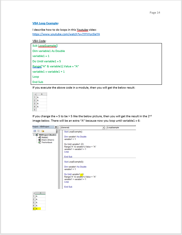
VBA Loop Example:
I describe how to do loops in this Youtube video: https://www.youtube.com/watch?v=7JYVVycGeYA
VBA Code:
Sub LoopExample()
Dim variable1 As Double
variable1 = 1
Do Until variable1 = 5
Range("A" & variable1).Value = "A"
variable1 = variable1 + 1
Loop
End Sub
If you execute the above code in a module, then you will get the below result:

If you change the = 5 to be > 5 like the below picture, then you will get the result in the 2nd image below. There will be an extra “A” because now you loop until variable1 = 6:
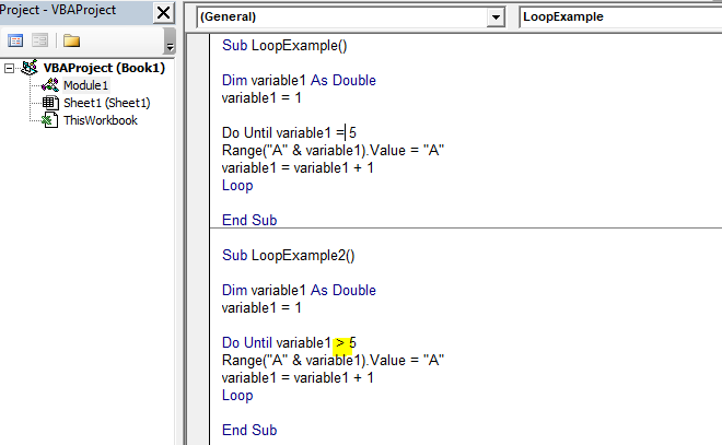

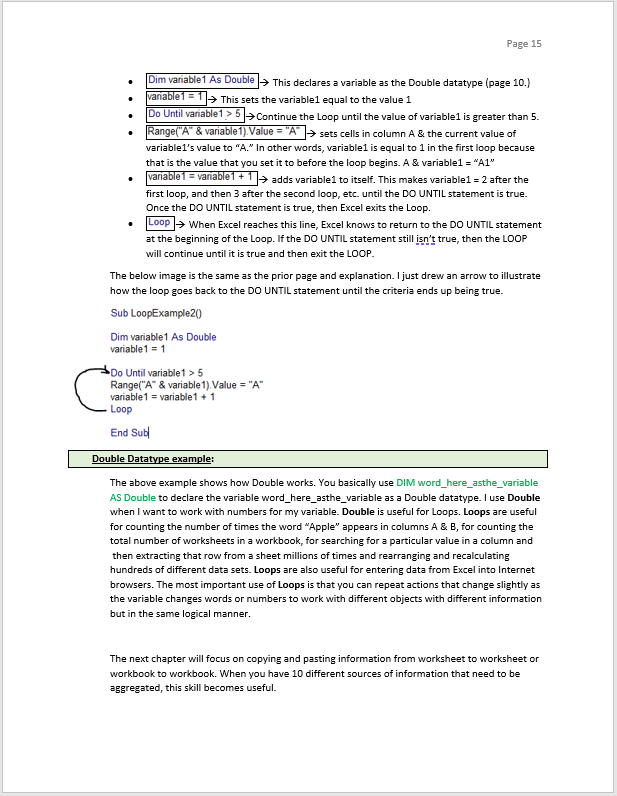
– This declares a variable as the Double datatype (page 10.)
– This sets the variable1 equal to the value 1
– Continue the Loop until the value of variable1 is greater than 5.
– sets cells in column A & the current value of variable1’s value to “A.” In other words, variable1 is equal to 1 in the first loop because that is the value that you set it to before the loop begins. A & variable1 = “A1”
– adds variable1 to itself. This makes variable1 = 2 after the first loop, and then 3 after the second loop, etc. until the DO UNTIL statement is true. Once the DO UNTIL statement is true, then Excel exits the Loop.
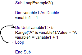
– When Excel reaches this line, Excel knows to return to the DO UNTIL statement at the beginning of the Loop. If the DO UNTIL statement still isn’t true, then the LOOP will continue until it is true and then exit the LOOP.
The below image is the same as the prior page and explanation. I just drew an arrow to illustrate how the loop goes back to the DO UNTIL statement until the criteria ends up being true.
Double Datatype example:
The above example shows how Double works. You basically use DIM word_here_asthe_variable AS Double to declare the variable word_here_asthe_variable as a Double datatype. I use Double when I want to work with numbers for my variable. Double is useful for Loops. Loops are useful for counting the number of times the word “Apple” appears in columns A & B, for counting the total number of worksheets in a workbook, for searching for a particular value in a column and then extracting that row from a sheet millions of times and rearranging and recalculating hundreds of different data sets. Loops are also useful for entering data from Excel into Internet browsers. The most important use of Loops is that you can repeat actions that change slightly as the variable changes words or numbers to work with different objects with different information but in the same logical manner.
The next chapter will focus on copying and pasting information from worksheet to worksheet or workbook to workbook. When you have 10 different sources of information that need to be aggregated, this skill becomes useful.

VBA Workbooks, Copy and Paste, Paths, Worksheets, & Modules Referencing Other Modules:
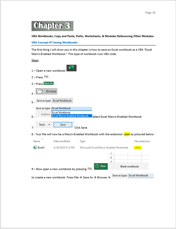
VBA Concept #7 Saving Workbooks:
The first thing I will show you in this chapter is how to save an Excel workbook as a VBA “Excel Macro-Enabled Workbook.” This type of workbook runs VBA code.
Steps:
Steps:
1 – Open a new workbook:
2 – Press
3 – Press
4 –
5 –
6 – Select Excel Macro-Enabled Workbook
7 – Click Save.
8 – Your file will now be a Macro-Enabled Workbook with the extension .xlsm as pictured below:

9 – Now open a new workbook by pressing
to create a new workbook. Press File à Save As – Browse –
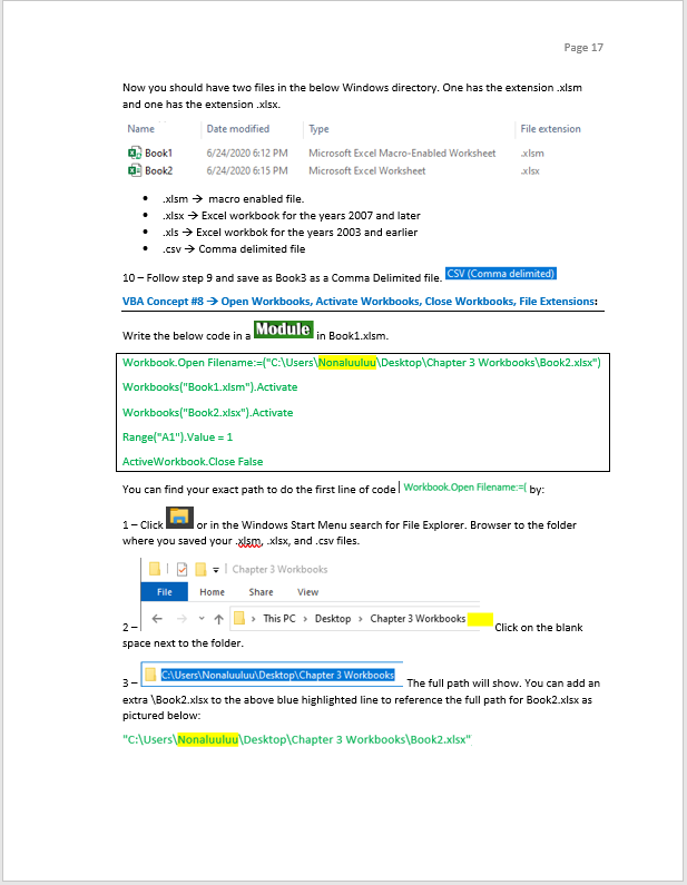
Now you should have two files in the below Windows directory. One has the extension .xlsm and one has the extension .xlsx.

- .xlsm – macro enabled file.
- .xlsx – Excel workbook for the years 2007 and later
- .xls – Excel workbok for the years 2003 and earlier
- .csv – Comma delimited file
10 – Follow step 9 and save as Book3 as a Comma Delimited file.
VBA Concept #8 – Open Workbooks, Activate Workbooks, Close Workbooks, File Extensions:
Write the below code in a in Book1.xlsm.
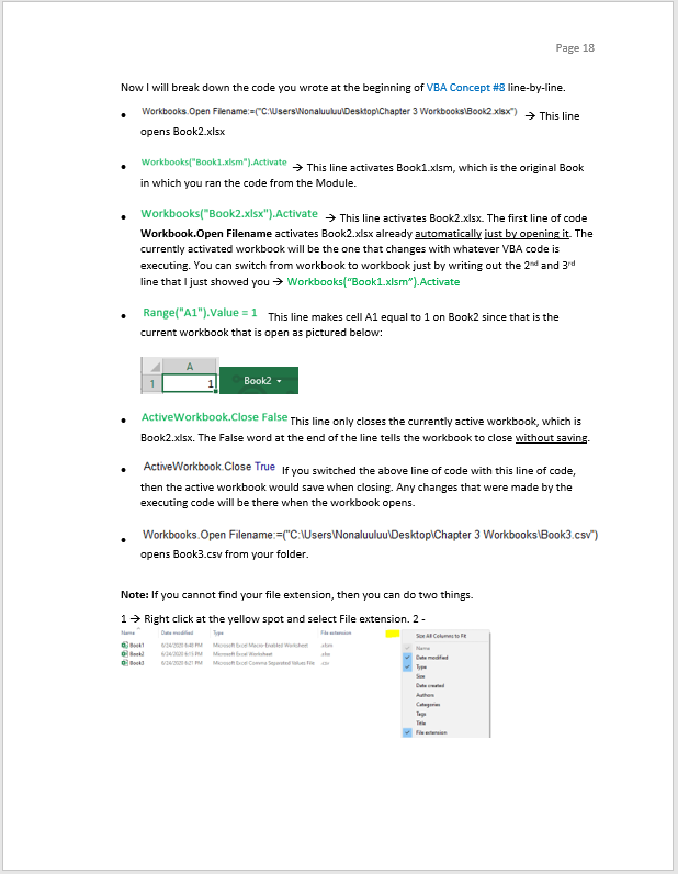
Workbooks.Open Filename:=("C:\Users\Nonaluuluu\Desktop\Chapter 3 Workbooks\Book2.xlsx")
Workbooks("Book1.xlsm").Activate
Workbooks("Book2.xlsx").Activate
Range("A1").Value = 1
ActiveWorkbook.Close False
You can find your exact path to do the first line of code by:
1 – Click or in the Windows Start Menu search for File Explorer. Browser to the folder where you saved your .xlsm, .xlsx, and .csv files.
2 – Click on the blank space next to the folder.
3 – The full path will show. You can add an extra \Book2.xlsx to the above blue highlighted line to reference the full path for Book2.xlsx as pictured below:

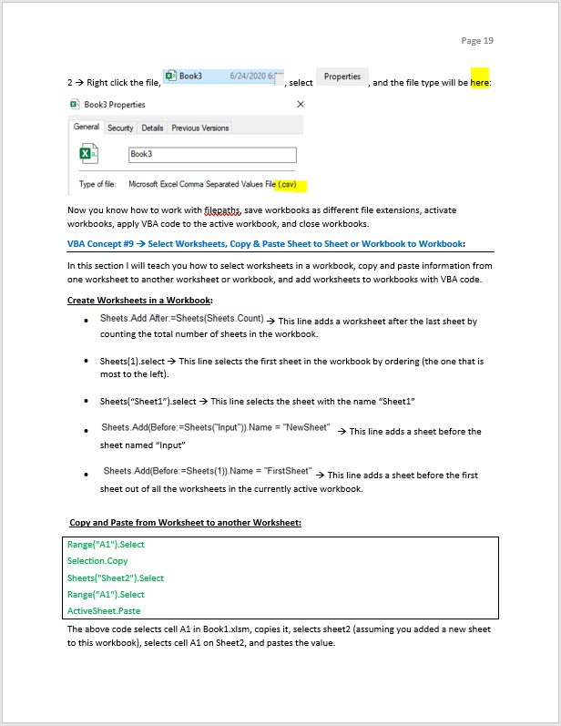
Now I will break down the code you wrote at the beginning of VBA Concept #8 line-by-line.
– This line opens Book2.xlsx
– This line activates Book1.xlsm, which is the original Book in which you ran the code from the Module.
– This line activates Book2.xlsx. The first line of code Workbooks.Open Filename activates Book2.xlsx already automatically just by opening it. The currently activated workbook will be the one that changes with whatever VBA code is executing. You can switch from workbook to workbook just by writing out the 2nd and 3rd line that I just showed you à Workbooks(“Book1.xlsm”).Activate
This line makes cell A1 equal to 1 on Book2 since that is the current workbook that is open as pictured below:


This line only closes the currently active workbook, which is Book2.xlsx. The False word at the end of the line tells the workbook to close without saving.
If you switched the above line of code with this line of code, then the active workbook would save when closing. Any changes that were made by the executing code will be there when the workbook opens.
opens Book3.csv from your folder.
Note: If you cannot find your file extension, then you can do two things.
1 – Right click at the yellow spot and select File extension. 2 –
2 – Right click the file, , select
, and the file type will be here:
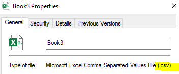
Now you know how to work with filepaths, save workbooks as different file extensions, activate workbooks, apply VBA code to the active workbook, and close workbooks.
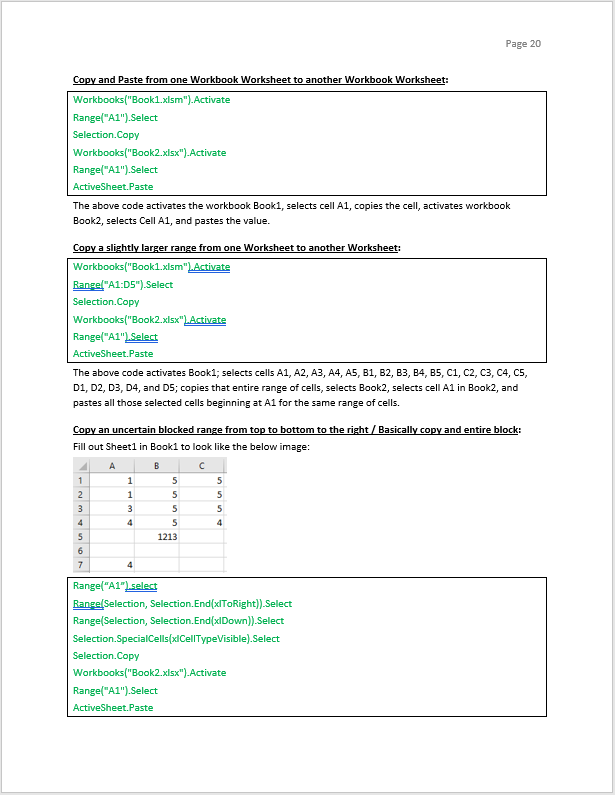
VBA Concept #9 – Select Worksheets, Copy & Paste Sheet to Sheet or Workbook to Workbook:
In this section I will teach you how to select worksheets in a workbook, copy and paste information from one worksheet to another worksheet or workbook, and add worksheets to workbooks with VBA code.
Create Worksheets in a Workbook:
– This line adds a worksheet after the last sheet by counting the total number of sheets in the workbook.
- Sheets(1).select – This line selects the first sheet in the workbook by ordering (the one that is most to the left).
- Sheets("Sheet1").select – This line selects the sheet with the name “Sheet1”
– This line adds a sheet before the sheet named “Input”
– This line adds a sheet before the first sheet out of all the worksheets in the currently active workbook.
Copy and Paste from Worksheet to another Worksheet:
Range("A1").Select
Selection.Copy
Sheets("Sheet2").Select
Range("A1").Select
ActiveSheet.Paste
The above code selects cell A1 in Book1.xlsm, copies it, selects sheet2 (assuming you added a new sheet to this workbook), selects cell A1 on Sheet2, and pastes the value.
Copy and Paste from one Workbook Worksheet to another Workbook Worksheet:
Workbooks("Book1.xlsm").Activate
Range("A1").Select
Selection.Copy
Workbooks("Book2.xlsx").Activate
Range("A1").Select
ActiveSheet.Paste
The above code activates the workbook Book1, selects cell A1, copies the cell, activates workbook Book2, selects Cell A1, and pastes the value.
Copy a slightly larger range from one Worksheet to another Worksheet:
Workbooks("Book1.xlsm").Activate
Range("A1:D5").Select
Selection.Copy
Workbooks("Book2.xlsx").Activate
Range("A1").Select
ActiveSheet.Paste
The above code activates Book1; selects cells A1, A2, A3, A4, A5, B1, B2, B3, B4, B5, C1, C2, C3, C4, C5, D1, D2, D3, D4, and D5; copies that entire range of cells, selects Book2, selects cell A1 in Book2, and pastes all those selected cells beginning at A1 for the same range of cells.
Copy an uncertain blocked range from top to bottom to the right / Basically copy and entire block:
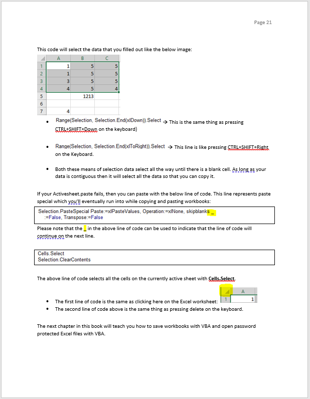
Fill out Sheet1 in Book1 to look like the below image:
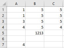
Range("A1").select
Range(Selection, Selection.End(xlToRight)).Select
Range(Selection, Selection.End(xlDown)).Select
Selection.SpecialCells(xlCellTypeVisible).Select
Selection.Copy
Workbooks("Book2.xlsx").Activate
Range("A1").Select
ActiveSheet.Paste
This code will select the data that you filled out like the below image:
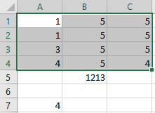
– This is the same thing as pressing CTRL+SHIFT+Down on the keyboard)
– This line is like pressing CTRL+SHIFT+Right on the Keyboard.
- Both these means of selection data select all the way until there is a blank cell. As long as your data is contiguous then it will select all the data so that you can copy it.
If your Activesheet.paste fails, then you can paste with the below line of code. This line represents paste special which you’ll eventually run into while copying and pasting workbooks. Paste special is useful when pasting a cell to get rid of the formula and keep only the value in the cell.

Please note that the _ in the above line of code can be used to indicate that the line of code will continue on the next line.

The above line of code selects all the cells on the currently active sheet with Cells.Select.
- The first line of code is the same as clicking here on the Excel worksheet:
- The second line of code above is the same thing as pressing delete on the keyboard.
The next chapter in this book will teach you how to save workbooks with VBA and open password protected Excel files with VBA.
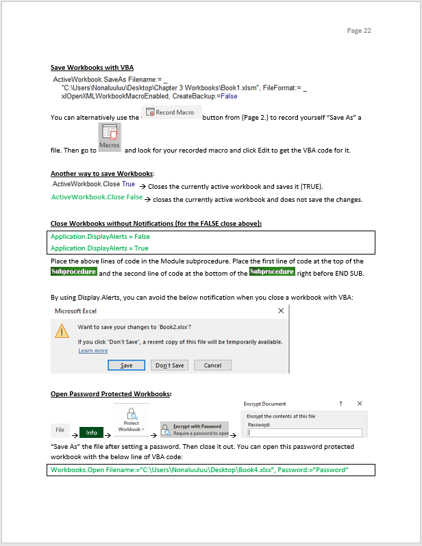
Save Workbooks with VBA

You can alternatively use the button from (Page 2.) to record yourself “Save As” a file. Then go to
and look for your recorded macro and click Edit to get the VBA code for it.
Another way to save Workbooks:
– Closes the currently active workbook and saves it (TRUE).
– closes the currently active workbook and does not save the changes.
Close Workbooks without Notifications (for the FALSE close above):
Application.DisplayAlerts = False
Application.DisplayAlerts = True
Place the above lines of code in the Module subprocedure. Place the first line of code at the top of the and the second line of code at the bottom of the
right before END SUB.
By using Display.Alerts, you can avoid the below notification when you close a workbook with VBA:

Open Password Protected Workbooks:
–
–
–
–
“Save As” the file after setting a password. Then close it out. You can open this password protected workbook with the below line of VBA code:
Workbooks.Open Filename:=”C:\Users\Nonaluuluu\Desktop\Book4.xlsx”, Password:=”Password”
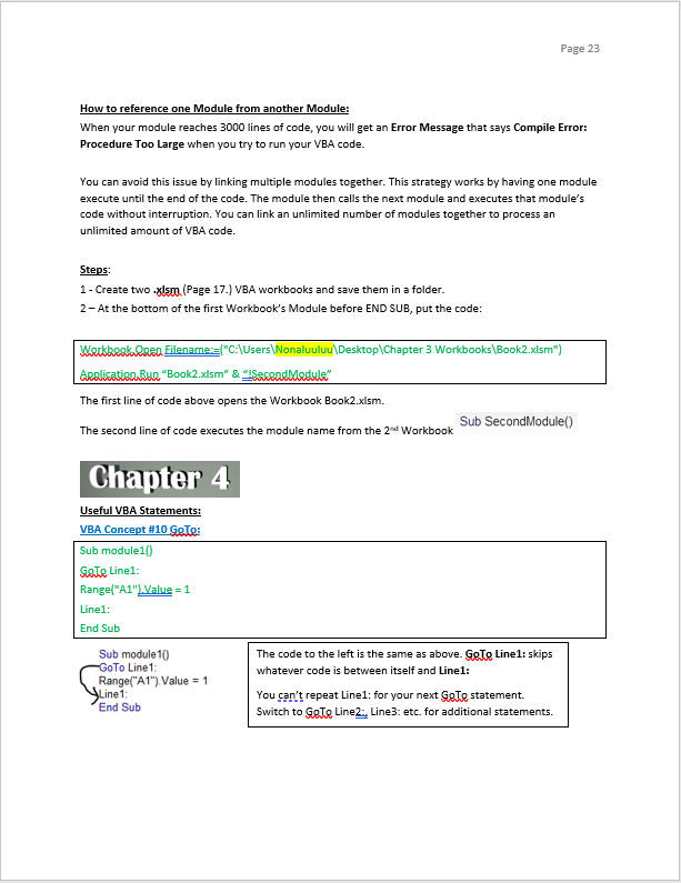
How to reference one Module from another Module:
When your module reaches 3000 lines of code, you will get an Error Message that says Compile Error: Procedure Too Large when you try to run your VBA code.
You can avoid this issue by linking multiple modules together. This strategy works by having one module execute until the end of the code. The module then calls the next module and executes that module’s code without interruption. You can link an unlimited number of modules together to process an unlimited amount of VBA code.
Steps:
1 – Create two .xlsm (Page 17.) VBA workbooks and save them in a folder.
2 – At the bottom of the first Workbook’s Module before END SUB, put the code:
Workbooks.Open Filename:=("C:\Users\Nonaluuluu\Desktop\Chapter 3 Workbooks\Book2.xlsm")
Application.Run "Book2.xlsm" & "!SecondModule"
The first line of code above opens the Workbook Book2.xlsm.
The second line of code executes the module name from the 2nd Workbook

Useful VBA Statements | GoTo, If, And, Or, Inputbox, Msgbox, Select Case:
VBA Concept #10 GoTo:
Sub module1()
GoTo Line1:
Range("A1").Value = 1
Line1:
End Sub

VBA Concept #11 If, Else, EndIf:
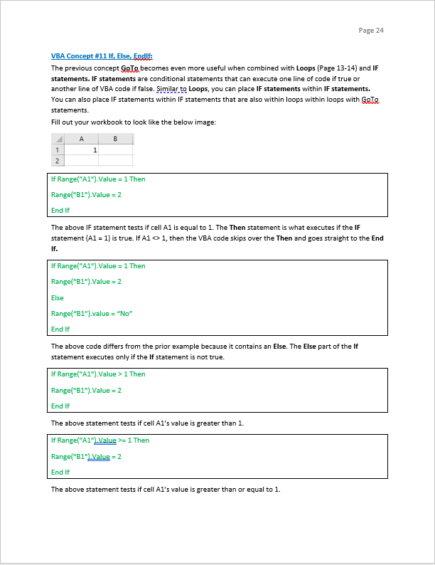
The previous concept GoTo becomes even more useful when combined with Loops (Page 13-14) and IF statements. IF statements are conditional statements that can execute one line of code if true or another line of VBA code if false. Similar to Loops, you can place IF statements within IF statements. You can also place IF statements within IF statements that are also within loops within loops with GoTo statements.
Fill out your workbook to look like the below image:
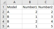
If Range("A1").Value = 1 Then
Range("B1").Value = 2
End If
The above IF statement tests if cell A1 is equal to 1. The Then statement is what executes if the IF statement (A1 = 1) is true. If A1 <> 1, then the VBA code skips over the Then and goes straight to the End If.
If Range("A1").Value = 1 Then
Range("B1").Value = 2
Else
Range("B1").value = "No"
End If
The above code differs from the prior example because it contains an Else. The Else part of the If statement executes only if the If statement is not true.
If Range("A1").Value > 1 Then
Range("B1").Value = 2
End If
The above statement tests if cell A1’s value is greater than 1.
If Range("A1").Value >= 1 Then
Range("B1").Value = 2
End If
The above statement tests if cell A1’s value is greater than or equal to 1.
If Range("A1").Value <> 1 Then
Range("B1").Value = 2
End If
The above statement tests if cell A1 does not equal 1.
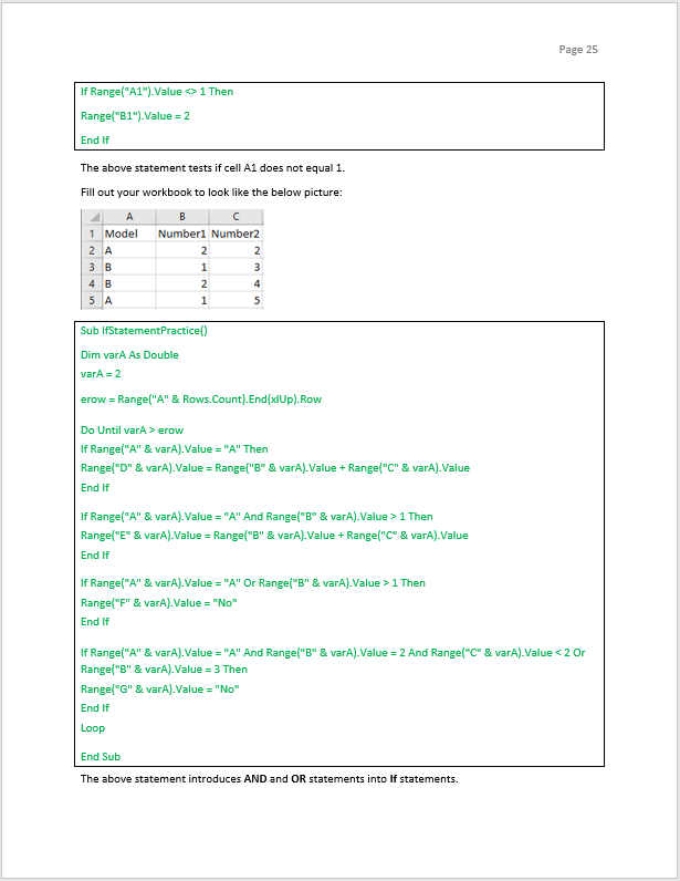
Fill out your workbook to look like the below picture:

Sub IfStatementPractice()
Dim varA As Double
varA = 2
erow = Range("A" & Rows.Count).End(xlUp).Row
Do Until varA > erow
If Range("A" & varA).Value = "A" Then
Range("D" & varA).Value = Range("B" & varA).Value + Range("C" & varA).Value
End If
If Range("A" & varA).Value = "A" And Range("B" & varA).Value > 1 Then
Range("E" & varA).Value = Range("B" & varA).Value + Range("C" & varA).Value
End If
If Range("A" & varA).Value = "A" Or Range("B" & varA).Value > 1 Then
Range("F" & varA).Value = "No"
End If
If Range("A" & varA).Value = "A" And Range("B" & varA).Value = 2 And Range("C" & varA).Value < 2 Or Range("B" & varA).Value = 3 Then
Range("G" & varA).Value = "No"
End If
Loop
End Sub
The above statement introduces AND and OR statements into If statements.
AND – can be used two, three, or four times in a single If statement. All of the ANDs must be true for the Then statement line to execute.
OR – Only one of the two statements in the IF statement needs to be true in order execute the Then statement.
AND/OR – When you combine multiple ANDs and a single OR statement, then only the OR statement needs to be true or all the ANDS need to be true. (This can be seen in the “G” value in the above example.
I like to combine If statements with Loops to fill the sheet with 1s and then section out the data based on whatever criteria I need by also using Filters, which I will show you in the next chapter.
VBA Concept #12 Inputbox:
Sub InputBoxPractice()
Dim ExlFileName As String
ExlFileName = InputBox("Enter old file's name")
ActiveWorkbook.SaveAs filename:= _
"C:\Users\Nonaluuluu\Desktop\VBATutorialCode Lessons\Inputbox\" & ExlFileName & ".xlsm" _
, FileFormat:=xlOpenXMLWorkbookMacroEnabled, CreateBackup:=False
End Sub
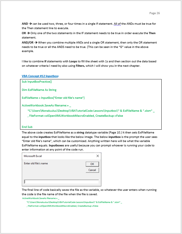
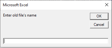
The above code creates ExlFileName as a string datatype variable (Page 10.) It then sets ExlFileName equal to the inputbox that looks like the below image. The below inputbox is the prompt the user sees “Enter old file’s name”, which can be customized. Anything written here will be what the variable ExlFileName equals. Inputboxes are useful because you can prompt whoever is running your code to enter information at any point of the code run.
The final line of code basically saves the file as the variable, so whatever the user enters when running the code is the file name of the file when the file is saved.

VBA Concept #13 Msgbox:
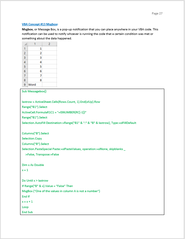
Msgbox, or Message Box, is a pop-up notification that you can place anywhere in your VBA code. This notification can be used to notify whoever is running the code that a certain condition was met or something about the data happened.
Sub Messagebox()
lastrow = ActiveSheet.Cells(Rows.Count, 1).End(xlUp).Row
Range("B1").Select
ActiveCell.FormulaR1C1 = "=ISNUMBER(RC[-1])"
Range("B1").Select
Selection.AutoFill Destination:=Range("B1" & ":" & "B" & lastrow), Type:=xlFillDefault
Columns("B").Select
Selection.Copy
Columns("B").Select
Selection.PasteSpecial Paste:=xlPasteValues, operation:=xlNone, skipblanks _
:=False, Transpose:=False
Dim x As Double
x = 1
Do Until x > lastrow
If Range("B" & x).Value = "False" Then
MsgBox ("One of the values in column A is not a number")
End If
x = x + 1
Loop
End Sub
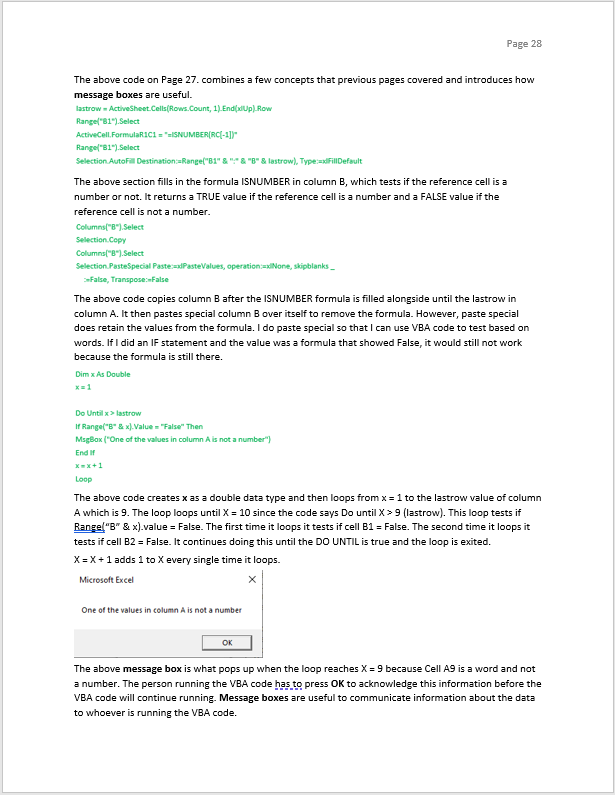
The above code on Page 27. combines a few concepts that previous pages covered and introduces how message boxes are useful.

The above section fills in the formula ISNUMBER in column B, which tests if the reference cell is a number or not. It returns a TRUE value if the reference cell is a number and a FALSE value if the reference cell is not a number.

The above code copies column B after the ISNUMBER formula is filled alongside until the lastrow in column A. It then pastes special column B over itself to remove the formula. However, paste special does retain the values from the formula. I do paste special so that I can use VBA code to test based on words. If I did an IF statement and the value was a formula that showed False, it would still not work because the formula is still there.
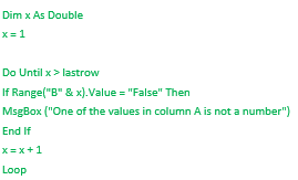
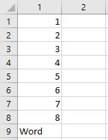
The above code creates x as a double data type and then loops from x = 1 to the lastrow value of column A which is 9. The loop loops until X = 10 since the code says Do until X > 9 (lastrow). This loop tests if Range(“B” & x).value = False. The first time it loops it tests if cell B1 = False. The second time it loops it tests if cell B2 = False. It continues doing this until the DO UNTIL is true and the loop is exited.
X = X + 1 adds 1 to X every single time it loops.
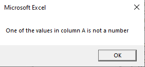
The above message box is what pops up when the loop reaches X = 9 because Cell A9 is a word and not a number. The person running the VBA code must press OK to acknowledge this information before the VBA code will continue running. Message boxes are useful to communicate information about the data to whoever is running the VBA code.
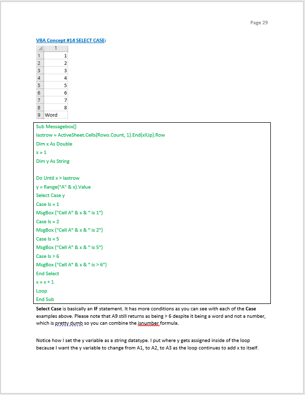
VBA Concept #14 SELECT CASE:

Sub Messagebox()
lastrow = ActiveSheet.Cells(Rows.Count, 1).End(xlUp).Row
Dim x As Double
x = 1
Dim y As String
Do Until x > lastrow
y = Range("A" & x).Value
Select Case y
Case Is = 1
MsgBox ("Cell A" & x & " is 1″)
Case Is = 2
MsgBox ("Cell A" & x & " is 2″)
Case Is = 5
MsgBox ("Cell A" & x & " is 5″)
Case Is > 6
MsgBox ("Cell A" & x & " is > 6″)
End Select
x = x + 1
Loop
End Sub
Select Case is basically an IF statement. It has more conditions as you can see with each of the Case examples above. Please note that A9 still returns as being > 6 despite it being a word and not a number, which is pretty dumb so you can combine the isnumber formula.
Notice how I set the y variable as a string datatype. I put where y gets assigned inside of the loop because I want the y variable to change from A1, to A2, to A3 as the loop continues to add x to itself.

VBA Filter, Advanced Filter, Pivot Table Filter Criteria:
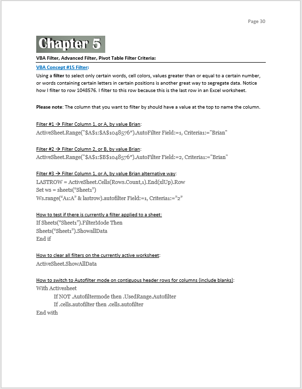
VBA Concept #15 Filter:
Using a filter to select only certain words, cell colors, values greater than or equal to a certain number, or words containing certain letters in certain positions is another great way to segregate data. Notice how I filter to row 1048576. I filter to this row because this is the last row in an Excel worksheet.
Please note: The column that you want to filter by should have a value at the top to name the column.
Filter #1 – Filter Column 1, or A, by value Brian:
ActiveSheet.Range("$A$1:$A$1048576″).AutoFilter Field:=1, Criteria1:="Brian"
Filter #2 – Filter Column 2, or B, by value Brian:
ActiveSheet.Range("$A$1:$B$1048576″).AutoFilter Field:=2, Criteria1:="Brian"
Filter #3 – Filter Column 1, or A, by value Brian alternative way:
LASTROW = ActiveSheet.Cells(Rows.Count,1).End(xlUp).Row
Set ws = sheets("Sheet1")
Ws.range("A1:A" & lastrow).autofilter Field:=1, Criteria1:="2″
How to test if there is currently a filter applied to a sheet:
If Sheets("Sheet1").FilterMode Then
Sheets("Sheet1").ShowallData
End if
How to clear all filters on the currently active worksheet:
ActiveSheet.ShowAllData
How to switch to Autofilter mode on contiguous header rows for columns (include blanks):
With Activesheet
If NOT .Autofiltermode then .UsedRange.Autofilter
If .cells.autofilter then .cells.autofilter
End with
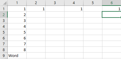
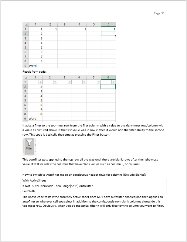
Result from code:
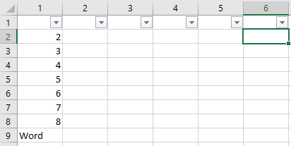
It adds a filter to the top-most row from the first column with a value to the right-most row/column with a value as pictured above. If the first value was in row 2, then it would add the filter ability to the second row. This code is basically the same as pressing the Filter button:

This autofilter gets applied to the top row all the way until there are blank rows after the right-most value. It still includes the columns that have blank values such as column 3, or column C.
How to switch to Autofilter mode on contiguous header rows for columns (Exclude Blanks):
With ActiveSheet
If Not .AutoFilterMode Then Range("A1").AutoFilter
End With
The above code tests if the currently active sheet does NOT have autofilter enabled and then applies an autofilter to whatever cell you select in addition to the contiguously non-blank columns alongside this top-most row. Obviously, when you do the actual filter it will only filter by the column you want to filter.
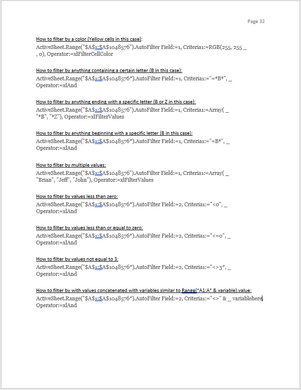
How to filter by a color (Yellow cells in this case):
ActiveSheet.Range("$A$1:$A$1048576").AutoFilter Field:=1, Criteria1:=RGB(255, 255 _
, 0), Operator:=xlFilterCellColor
How to filter by anything containing a certain letter (B in this case):
ActiveSheet.Range("$A$1:$A$1048576″).AutoFilter Field:=1, Criteria1:="=*B*", _
Operator:=xlAnd
How to filter by anything ending with a specific letter (B or Z in this case):
ActiveSheet.Range("$A$1:$A$1048576").AutoFilter Field:=1, Criteria1:=Array( _
"*B", "*Z"), Operator:=xlFilterValues
How to filter by anything beginning with a specific letter (B in this case):
ActiveSheet.Range("$A$1:$A$1048576″).AutoFilter Field:=1, Criteria1:="=B*", _
Operator:=xlAnd
How to filter by multiple values:
ActiveSheet.Range("$A$1:$A$1048576").AutoFilter Field:=1, Criteria1:=Array( _
"Brian", "Jeff", "John"), Operator:=xlFilterValues
How to filter by values less than zero:
ActiveSheet.Range("$A$1:$A$1048576″).AutoFilter Field:=2, Criteria1:="<0", _ Operator:=xlAnd
How to filter by values less than or equal to zero:
ActiveSheet.Range("$A$1:$A$1048576″).AutoFilter Field:=2, Criteria1:="<=0", _ Operator:=xlAnd
How to filter by values not equal to 3:
ActiveSheet.Range("$A$1:$A$1048576″).AutoFilter Field:=2, Criteria1:="<>3″, _ Operator:=xlAnd
How to filter by with values concatenated with variables similar to Range(“A1:A” & variable).value:
ActiveSheet.Range("$A$1:$A$1048576″).AutoFilter Field:=2, Criteria1:="<>" & _ variablehere, Operator:=xlAnd
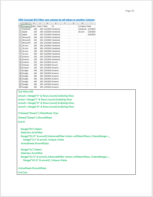
VBA Concept #15 Filter one column by all values in another Column:
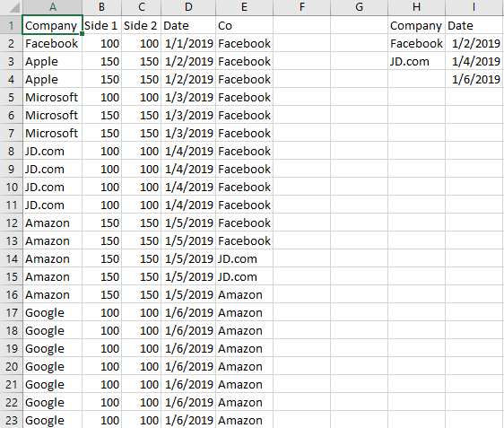
Sub Macro3()
erowA = Range("A" & Rows.Count).End(xlUp).Row
erowI = Range("I" & Rows.Count).End(xlUp).Row
erowD = Range("D" & Rows.Count).End(xlUp).Row
erowH = Range("H" & Rows.Count).End(xlUp).Row
If Sheets("Sheet1").FilterMode Then
Sheets("Sheet1").ShowAllData
End If
Range("D1").Select
Selection.AutoFilter
Range("D1:D" & erowD).AdvancedFilter Action:=xlFilterInPlace, CriteriaRange:= _
Range("I1:I" & erowI), Unique:=False
ActiveSheet.ShowAllData
Range("A1").Select
Selection.AutoFilter
Range("A1:A" & erowA).AdvancedFilter Action:=xlFilterInPlace, CriteriaRange:= _
Range("H1:H" & erowH), Unique:=False
ActiveSheet.ShowAllData
End Sub
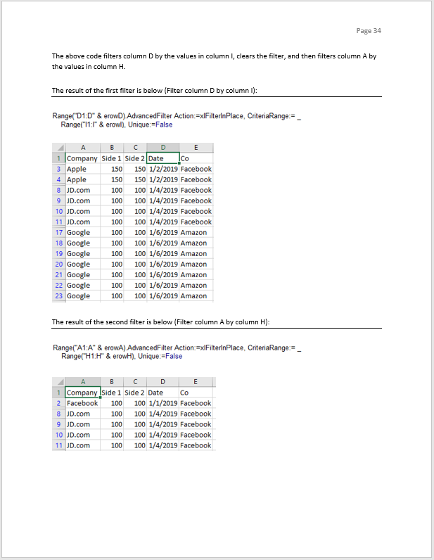
The above code filters column D by the values in column I, clears the filter, and then filters column A by the values in column H.
The result of the first filter is below (Filter column D by column I):

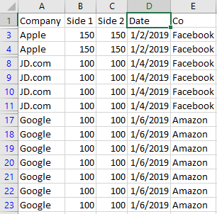
The result of the second filter is below (Filter column A by column H):

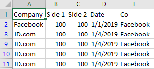
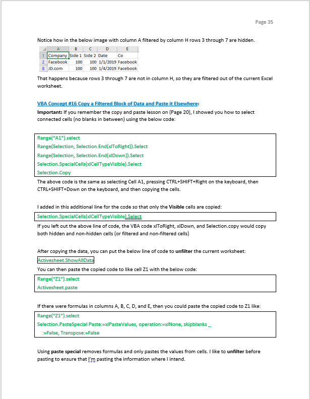
Notice how in the below image with column A filtered by column H rows 3 through 7 are hidden.

That happens because rows 3 through 7 are not in column H, so they are filtered out of the current Excel worksheet.
VBA Concept #16 Copy a Filtered Block of Data and Paste it Elsewhere:
Important: If you remember the copy and paste lesson on (Page 20), I showed you how to select connected cells (no blanks in between) using the below code:
Range("A1").select
Range(Selection, Selection.End(xlToRight)).Select
Range(Selection, Selection.End(xlDown)).Select
Selection.SpecialCells(xlCellTypeVisible).Select
Selection.Copy
The above code is the same as selecting Cell A1, pressing CTRL+SHIFT+Right on the keyboard, then CTRL+SHIFT+Down on the keyboard, and then copying the cells.
I added in this additional line for the code so that only the Visible cells are copied:
Selection.SpecialCells(xlCellTypeVisible).Select
If you left out the above line of code, the VBA code xlToRight, xlDown, and Selection.copy would copy both hidden and non-hidden cells (or filtered and non-filtered cells)
After copying the data, you can put the below line of code to unfilter the current worksheet:
Activesheet.ShowAllData
You can then paste the copied code to like cell Z1 with the below code:
Range("Z1").select
Activesheet.paste
If there were formulas in columns A, B, C, D, and E, then you could paste the copied code to Z1 like:
Range("Z1").select
Selection.PasteSpecial Paste:=xlPasteValues, operation:=xlNone, skipblanks _
:=False, Transpose:=False
Using paste special removes formulas and only pastes the values from cells. I like to unfilter before pasting to ensure that I’m pasting the information where I intend.
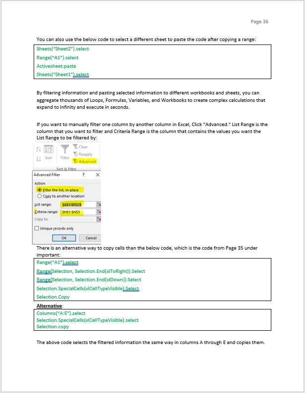
You can also use the below code to select a different sheet to paste the code after copying a range:
Sheets("Sheet2").select
Range("A1").select
Activesheet.paste
Sheets("Sheet1").select
By filtering information and pasting selected information to different workbooks and sheets, you can aggregate thousands of Loops, Formulas, Variables, and Workbooks to create complex calculations that expand to infinity and execute in seconds.
If you want to manually filter one column by another column in Excel, Click "Advanced." List Range is the column that you want to filter and Criteria Range is the column that contains the values you want the List Range to be filtered by:
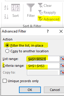
There is an alternative way to copy cells than the below code, which is the code from Page 35 under important:
Range("A1").select
Range(Selection, Selection.End(xlToRight)).Select
Range(Selection, Selection.End(xlDown)).Select
Selection.SpecialCells(xlCellTypeVisible).Select
Selection.Copy
Alternative:
Columns("A:E").select
Selection.SpecialCells(xlCellTypeVisible).select
Selection.copy
The above code selects the filtered information the same way in columns A through E and copies them.
Alternative #2:
LASTROW = ActiveSheet.Cells(Rows.Count,1).End(xlUp).Row
LASTROW2 = ActiveSheet.Cells(Rows.Count,5).End(xlUp).Row
Range("A1:A" & Lastrow & ":" & "E1:E" & lastrow2).select
Selection.SpecialCells(xlCellTypeVisible).select
Selection.copy
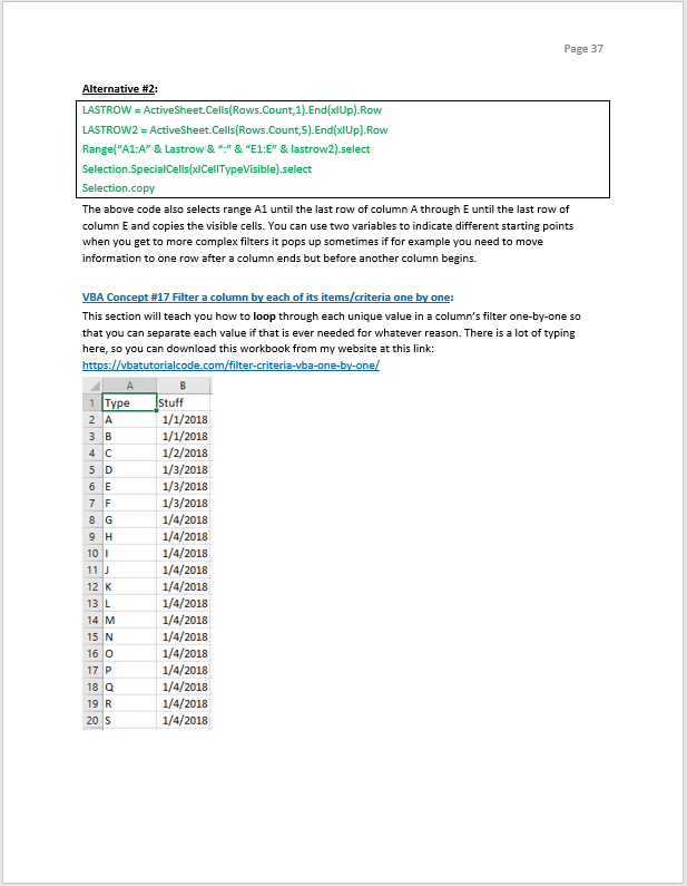
The above code also selects range A1 until the last row of column A through E until the last row of column E and copies the visible cells. You can use two variables to indicate different starting points when you get to more complex filters it pops up sometimes if for example you need to move information to one row after a column ends but before another column begins.
VBA Concept #17 Filter a column by each of its items/criteria one by one:
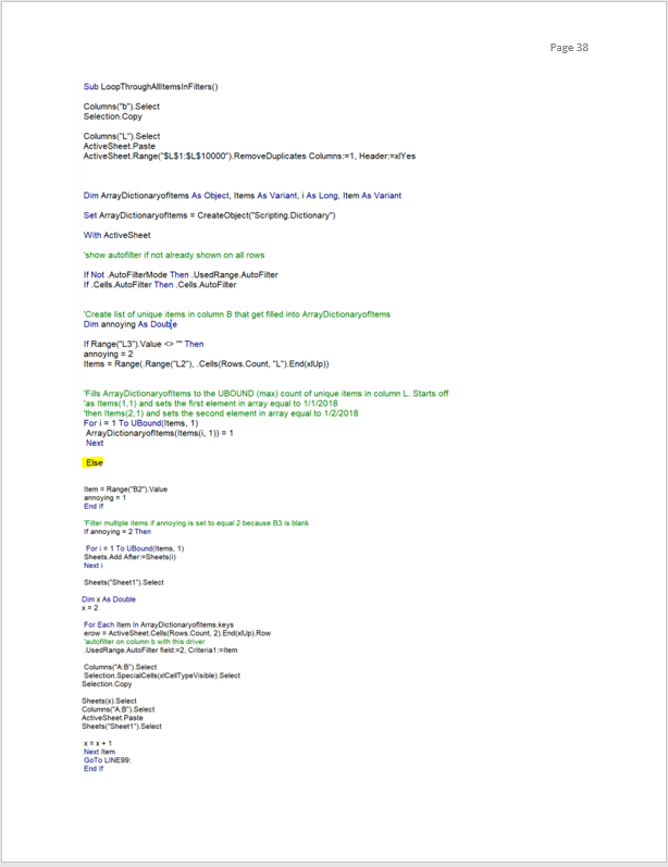
This section will teach you how to loop through each unique value in a column’s filter one-by-one so that you can separate each value if that is ever needed for whatever reason. There is a lot of typing here, so you can download this workbook from my website at this link: https://vbatutorialcode.com/filter-criteria-vba-one-by-one/
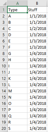
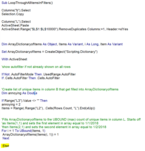
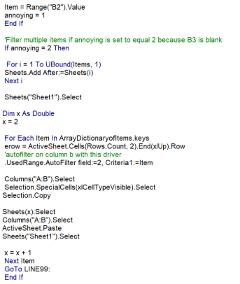
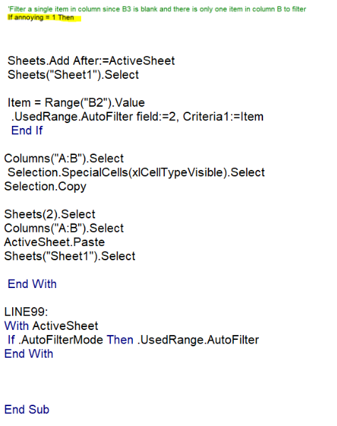
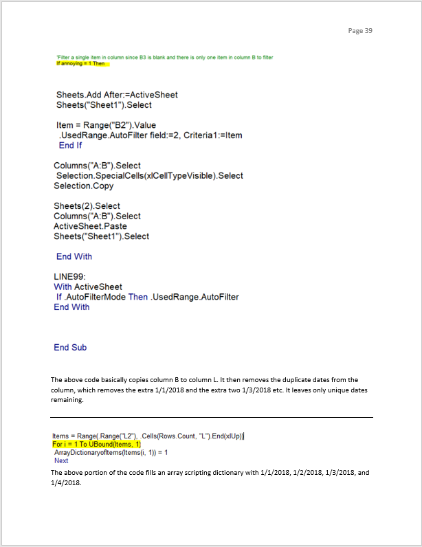
The above code basically copies column B to column L. It then removes the duplicate dates from the column, which removes the extra 1/1/2018 and the extra two 1/3/2018 etc. It leaves only unique dates remaining.

The above portion of the code fills an array scripting dictionary with 1/1/2018, 1/2/2018, 1/3/2018, and 1/4/2018.

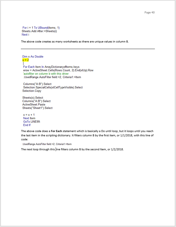
The above code creates as many worksheets as there are unique values in column B.
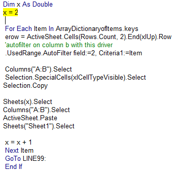
The above code does a For Each statement which is basically a Do until loop, but it loops until you reach the last item in the scripting dictionary. It filters column B by the first item, or 1/1/2018, with this line of code:

The next loop through this line filters column B by the second Item, or 1/2/2018.
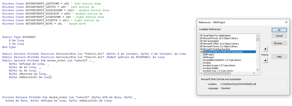


XY Coordinate Excel VBA

 VBA Tutorial Code


