VBA Excel Filter Lesson All Items and Pivot Tables

This page will teach you how to do every type of filtering in Excel with VBA. Notice how I filter to row 1048576. I filter to this row because this is the last row in an Excel worksheet. If you don't know this…. the _ at the end of a line indicates that the code continues on the next line.

Please note: The column that you want to filter by should have a value at the top to name the column.

Filter #1 – Filter Column 1, or A, by value Brian:

ActiveSheet.Range("$A$1:$A$1048576″).AutoFilter Field:=1, Criteria1:="Brian"

Filter #2 – Filter Column 2, or B, by value Brian:

ActiveSheet.Range("$A$1:$B$1048576″).AutoFilter Field:=2, Criteria1:="Brian"

Filter #3 – Filter Column 1, or A, by value Brian alternative way:

LASTROW = ActiveSheet.Cells(Rows.Count,1).End(xlUp).Row
Set ws = sheets("Sheet1")
Ws.range("A1:A" & lastrow).autofilter Field:=1, Criteria1:="2"

How to test if there is currently a filter applied to a sheet:

If Sheets("Sheet1").FilterMode Then
Sheets("Sheet1").ShowallData
End if

How to clear all filters on the currently active worksheet:

ActiveSheet.ShowAllData

How to switch to Autofilter mode on contiguous header rows for columns (include blanks):

With Activesheet
	If NOT .Autofiltermode then .UsedRange.Autofilter
	If .cells.autofilter then .cells.autofilter
End with

It adds a filter to the top-most row from the first column with a value to the right-most row/column with a value as pictured above. If the first value was in row 2, then it would add the filter ability to the second row. This code is basically the same as pressing the Filter button:

This autofilter gets applied to the top row all the way until there are blank rows after the right-most value. It still includes the columns that have blank values such as column 3, or column C.

How to switch to Autofilter mode on contiguous header rows for columns (Exclude Blanks):

With ActiveSheet
If Not .AutoFilterMode Then Range("A1").AutoFilter
End With

The above code tests if the currently active sheet does NOT have autofilter enabled and then applies an autofilter to whatever cell you select in addition to the contiguously non-blank columns alongside this top-most row. Obviously, when you do the actual filter it will only filter by the column you want to filter.

How to filter by a color (Yellow cells in this case):

ActiveSheet.Range("$A$1:$A$1048576").AutoFilter Field:=1, Criteria1:=RGB(255, 255 _
, 0), Operator:=xlFilterCellColor

How to filter by anything containing a certain letter (B in this case):

ActiveSheet.Range("$A$1:$A$1048576").AutoFilter Field:=1, Criteria1:="=*B*", _
Operator:=xlAnd

How to filter by anything ending with a specific letter (B or Z in this case):

ActiveSheet.Range("$A$1:$A$1048576").AutoFilter Field:=1, Criteria1:=Array( _
"*B", "*Z"), Operator:=xlFilterValues

How to filter by anything beginning with a specific letter (B in this case):

ActiveSheet.Range("$A$1:$A$1048576").AutoFilter Field:=1, Criteria1:="=B*", _
Operator:=xlAnd

How to filter by multiple values:

ActiveSheet.Range("$A$1:$A$1048576").AutoFilter Field:=1, Criteria1:=Array( _
"Brian", "Jeff", "John"), Operator:=xlFilterValues

How to filter by values less than zero:

ActiveSheet.Range("$A$1:$A$1048576").AutoFilter Field:=2, Criteria1:="<0", _ Operator:=xlAnd

How to filter by values less than or equal to zero:

ActiveSheet.Range("$A$1:$A$1048576").AutoFilter Field:=2, Criteria1:="<=0", _ Operator:=xlAnd

How to filter by values not equal to 3:

ActiveSheet.Range("$A$1:$A$1048576").AutoFilter Field:=2, Criteria1:="<>3", _ Operator:=xlAnd

How to filter by with values concatenated with variables similar to Range(“A1:A” & variable).value:

ActiveSheet.Range("$A$1:$A$1048576").AutoFilter Field:=2, Criteria1:="<>" & _ variablehere, Operator:=xlAnd

Filter a column A by column H, then column D by I:

Sub Macro3()
erowA = Range("A" & Rows.Count).End(xlUp).Row
erowI = Range("I" & Rows.Count).End(xlUp).Row
erowD = Range("D" & Rows.Count).End(xlUp).Row
erowH = Range("H" & Rows.Count).End(xlUp).Row

If Sheets("Sheet1").FilterMode Then
Sheets("Sheet1").ShowAllData
End If

    Range("D1").Select
    Selection.AutoFilter
    Range("D1:D" & erowD).AdvancedFilter Action:=xlFilterInPlace, CriteriaRange:= _
        Range("I1:I" & erowI), Unique:=False
    ActiveSheet.ShowAllData
    
    Range("A1").Select
    Selection.AutoFilter
    Range("A1:A" & erowA).AdvancedFilter Action:=xlFilterInPlace, CriteriaRange:= _
        Range("H1:H" & erowH), Unique:=False
   
ActiveSheet.ShowAllData
End Sub

The above code filters column D by the values in column I, clears the filter, and then filters column A by the values in column H.

VBA Concept #16 Copy a Filtered Block of Data and Paste it Elsewhere:

Important: If you remember the copy and paste lesson on (Page 20 of my FREE BOOK), I showed you how to select connected cells (no blanks in between) using the below code:

Range("A1").select
Range(Selection, Selection.End(xlToRight)).Select
Range(Selection, Selection.End(xlDown)).Select
Selection.SpecialCells(xlCellTypeVisible).Select
Selection.Copy

The above code is the same as selecting Cell A1, pressing CTRL+SHIFT+Right on the keyboard, then CTRL+SHIFT+Down on the keyboard, and then copying the cells.

I added in this additional line for the code so that only the Visible cells are copied:

Selection.SpecialCells(xlCellTypeVisible).Select

If you left out the above line of code, the VBA code xlToRight, xlDown, and Selection.copy would copy both hidden and non-hidden cells (or filtered and non-filtered cells)

After copying the data, you can put the below line of code to unfilter the current worksheet:

Activesheet.ShowAllData

You can then paste the copied code to like cell Z1 with the below code:

Range("Z1").select
Activesheet.paste

If there were formulas in columns A, B, C, D, and E, then you could paste the copied code to Z1 like:

Range("Z1").select
Selection.PasteSpecial Paste:=xlPasteValues, operation:=xlNone, skipblanks _
    :=False, Transpose:=False

Using paste special removes formulas and only pastes the values from cells. I like to unfilter before pasting to ensure that I’m pasting the information where I intend.

You can also use the below code to select a different sheet to paste the code after copying a range:

Sheets("Sheet2").select
Range(“A1”).select
Activesheet.paste
Sheets("Sheet1").select

By filtering information and pasting selected information to different workbooks and sheets, you can aggregate thousands of Loops, Formulas, Variables, and Workbooks to create complex calculations that expand to infinity and execute in seconds.

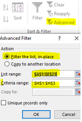
If you want to manually filter one column by another column in Excel, Click "Advanced." List Range is the column that you want to filter and Criteria Range is the column that contains the values you want the List Range to be filtered by:

There is an alternative way to copy cells than the below code, which is the code from Page 35 under important:

Range("A1").select
Range(Selection, Selection.End(xlToRight)).Select
Range(Selection, Selection.End(xlDown)).Select
Selection.SpecialCells(xlCellTypeVisible).Select
Selection.Copy

Alternative:

Columns("A:E").select
Selection.SpecialCells(xlCellTypeVisible).select
Selection.copy

The above code selects the filtered information the same way in columns A through E and copies them.

Alternative #2:

LASTROW = ActiveSheet.Cells(Rows.Count,1).End(xlUp).Row
LASTROW2 = ActiveSheet.Cells(Rows.Count,5).End(xlUp).Row
Range("A1:A" & Lastrow & ":" & "E1:E" & lastrow2).select
Selection.SpecialCells(xlCellTypeVisible).select
Selection.copy

The above code also selects range A1 until the last row of column A through E until the last row of column E and copies the visible cells. You can use two variables to indicate different starting points when you get to more complex filters it pops up sometimes if for example you need to move information to one row after a column ends but before another column begins.

VBA Concept #17 Filter a column by each of its items/criteria one by one:

This section will teach you how to loop through each unique value in a column’s filter one-by-one so that you can separate each value if that is ever needed for whatever reason. There is a lot of typing here, so you can download this workbook from my website at this link: https://vbatutorialcode.com/filter-criteria-vba-one-by-one/

Sub LoopThroughAllItemsInFilters()

Columns("b").Select
Selection.Copy

Columns("L").Select
ActiveSheet.Paste
ActiveSheet.Range("$L$1:$L$10000").RemoveDuplicates Columns:=1, Header:=xlYes



Dim ArrayDictionaryofItems As Object, Items As Variant, i As Long, Item As Variant

Set ArrayDictionaryofItems = CreateObject("Scripting.Dictionary")

With ActiveSheet

'show autofilter if not already shown on all rows

If Not .AutoFilterMode Then .UsedRange.AutoFilter
If .Cells.AutoFilter Then .Cells.AutoFilter


'Create list of unique items in column B that get filled into ArrayDictionaryofItems
Dim annoying As Double

If Range("B3").Value <> "" Then
annoying = 2
Items = Range(.Range("L2"), .Cells(Rows.Count, "L").End(xlUp))


'Fills ArrayDictionaryofItems to the UBOUND (max) count of unique items in column L. Starts off
'as Items(1,1) and sets the first element in array equal to 1/1/2018
'then Items(2,1) and sets the second element in array equal to 1/2/2018
For i = 1 To UBound(Items, 1)
 ArrayDictionaryofItems(Items(i, 1)) = 1
 Next
 
 Else
 
 Item = Range("B2").Value
 annoying = 1
 End If
 
 'Filter multiple items if annoying is set to equal 2 because B3 is blank
 If annoying = 2 Then
 
  For i = 1 To UBound(Items, 1)
 Sheets.Add After:=Sheets(i)
 Next i
 
 Sheets("Sheet1").Select

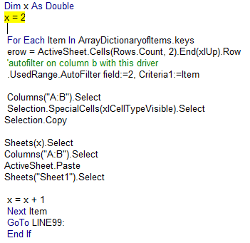
Dim x As Double
x = 2
 
 For Each Item In ArrayDictionaryofItems.keys
 erow = ActiveSheet.Cells(Rows.Count, 2).End(xlUp).Row
 'autofilter on column b with this driver
 .UsedRange.AutoFilter field:=2, Criteria1:=Item
 
 Columns("A:B").Select
 Selection.SpecialCells(xlCellTypeVisible).Select
Selection.Copy

Sheets(x).Select
Columns("A:B").Select
ActiveSheet.Paste
Sheets("Sheet1").Select

 x = x + 1
 Next Item
 GoTo LINE99:
 End If
 
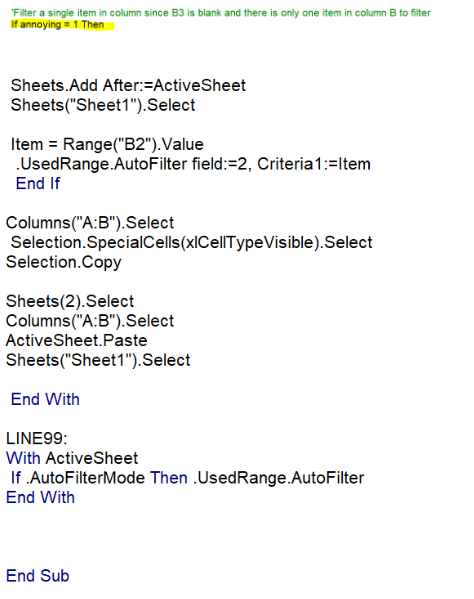
 'Filter a single item in column since B3 is blank and there is only one item in column B to filter
 If annoying = 1 Then
 
 Sheets.Add After:=ActiveSheet
 Sheets("Sheet1").Select
 
 Item = Range("B2").Value
  .UsedRange.AutoFilter field:=2, Criteria1:=Item
  End If

Columns("A:B").Select
 Selection.SpecialCells(xlCellTypeVisible).Select
Selection.Copy

Sheets(2).Select
Columns("A:B").Select
ActiveSheet.Paste
Sheets("Sheet1").Select
 
 End With
 
LINE99:
With ActiveSheet
 If .AutoFilterMode Then .UsedRange.AutoFilter
End With



End Sub

---

Breakdown of code:

The above code basically copies column B to column L. It then removes the duplicate dates from the column, which removes the extra 1/1/2018 and the extra two 1/3/2018 etc. It leaves only unique dates remaining.

---

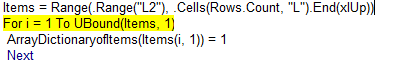
The above portion of the code fills an array scripting dictionary with 1/1/2018, 1/2/2018, 1/3/2018, and 1/4/2018. 

---

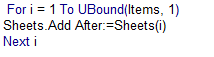
The above code creates as many worksheets as there are unique values in column B.

---

The above code does a For Each statement which is basically a Do until loop, but it loops until you reach the last item in the scripting dictionary. It filters column B by the first item, or 1/1/2018, with this line of code:

---

The next loop through this line filters column B by the second Item, or 1/2/2018.

---

Pivot table VBA Code loop through each item:

Sub LoopThroughFilters()

Dim annoying As Double

Dim driversdict As Object, drivers As Variant, i As Long, Driver As Variant

Set driversdict = CreateObject("Scripting.Dictionary")

With ActiveSheet

'puts autofilter on all columns
If Not .AutoFilterMode Then .UsedRange.AutoFilter
If .Cells.AutoFilter Then .Cells.AutoFilter

'Create list of unique things to filter by in column P

If Range("P3").Value <> "" Then
annoying = 2


drivers = Range(.Range("P2"), .Cells(Rows.Count, "P").End(xlUp))
For i = 1 To UBound(drivers, 1)
driversdict(drivers(i, 1)) = 1
counts = counts + 1
Next

Else

Driver = Range("P2").Value
annoying = 1
End If
End With

Sheets("Sheet2").Select
With ActiveSheet.PivotTables("Pivottable1").PivotFields("Date")
.Orientation = xlPageField
.Position = 1
End With
ActiveSheet.PivotTables("Pivottable1").PivotFields("Date").CurrentPage = _
"(All)"

Dim counter2 As Double
counter2 = 1

Dim key As Double
key = 1

For Each Driver In driversdict.keys

If key = 2 Then
GoTo line80:
End If

With ActiveSheet.PivotTables("Pivottable1").PivotFields("Date")
ActiveSheet.PivotTables("Pivottable1").PivotFields("Date").CurrentPage = _
"(All)"

With ActiveSheet.PivotTables("Pivottable1").PivotFields("Date")
For i = 1 To .PivotItems.Count
If i = ActiveSheet.PivotTables("Pivottable1").PivotFields("Date").PivotItems.Count Then
GoTo line6:
End If

.PivotItems(i).Visible = False
Next

line6:
End With

ActiveSheet.PivotTables("Pivottable1").PivotFields("Date"). _
EnableMultiplePageItems = True
line80:

With ActiveSheet.PivotTables("Pivottable1").PivotFields("Date")
.PivotItems(Driver).Visible = True
End With
If key = 2 Then
With ActiveSheet.PivotTables("Pivottable1").PivotFields("Date")
.PivotItems(counter2).Visible = False
End With
counter2 = counter2 + 1
End If

If key <> 2 Then
.PivotItems(i).Visible = False
key = 2
End If
End With

Next






End Sub